Rows: 601 Columns: 8
── Column specification ────────────────────────────────────────────────────────
Delimiter: ","
chr (2): game1, genre
dbl (6): year, totalearn, offlineearn, percent, totallayer, tournament

ℹ Use `spec()` to retrieve the full column specification for this data.
ℹ Specify the column types or set `show_col_types = FALSE` to quiet this message.
Rows: 9731 Columns: 5
── Column specification ────────────────────────────────────────────────────────
Delimiter: ","
chr  (1): game2
dbl  (3): earn, player, tournament
date (1): date

ℹ Use `spec()` to retrieve the full column specification for this data.
ℹ Specify the column types or set `show_col_types = FALSE` to quiet this message.
Data Analysis
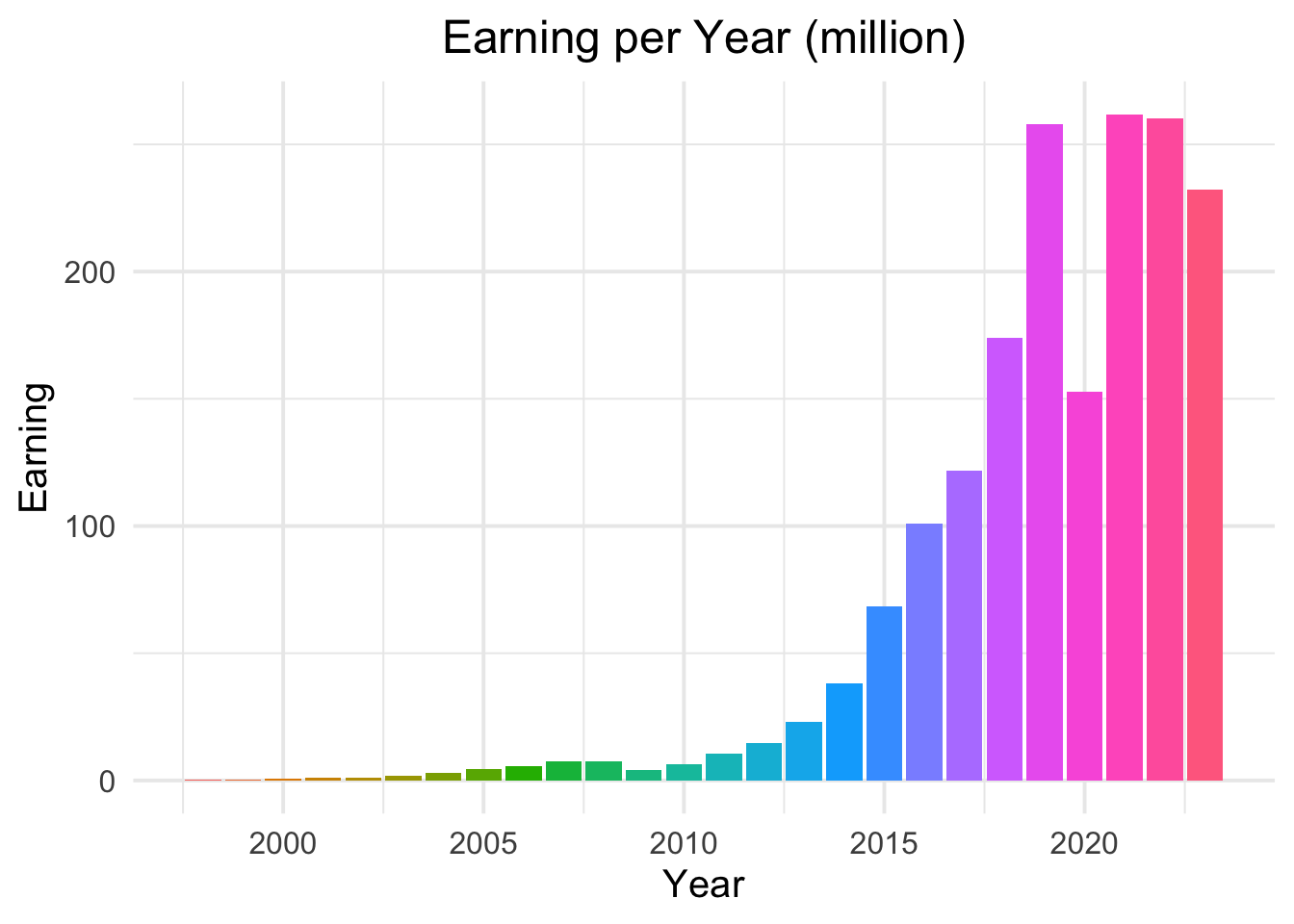
Earning per Year
Q1 asks the earning per year. To answer this question, I first extracted the year from the date column in the dataset. Then, I grouped the data by year and calculated the total earnings for each year.
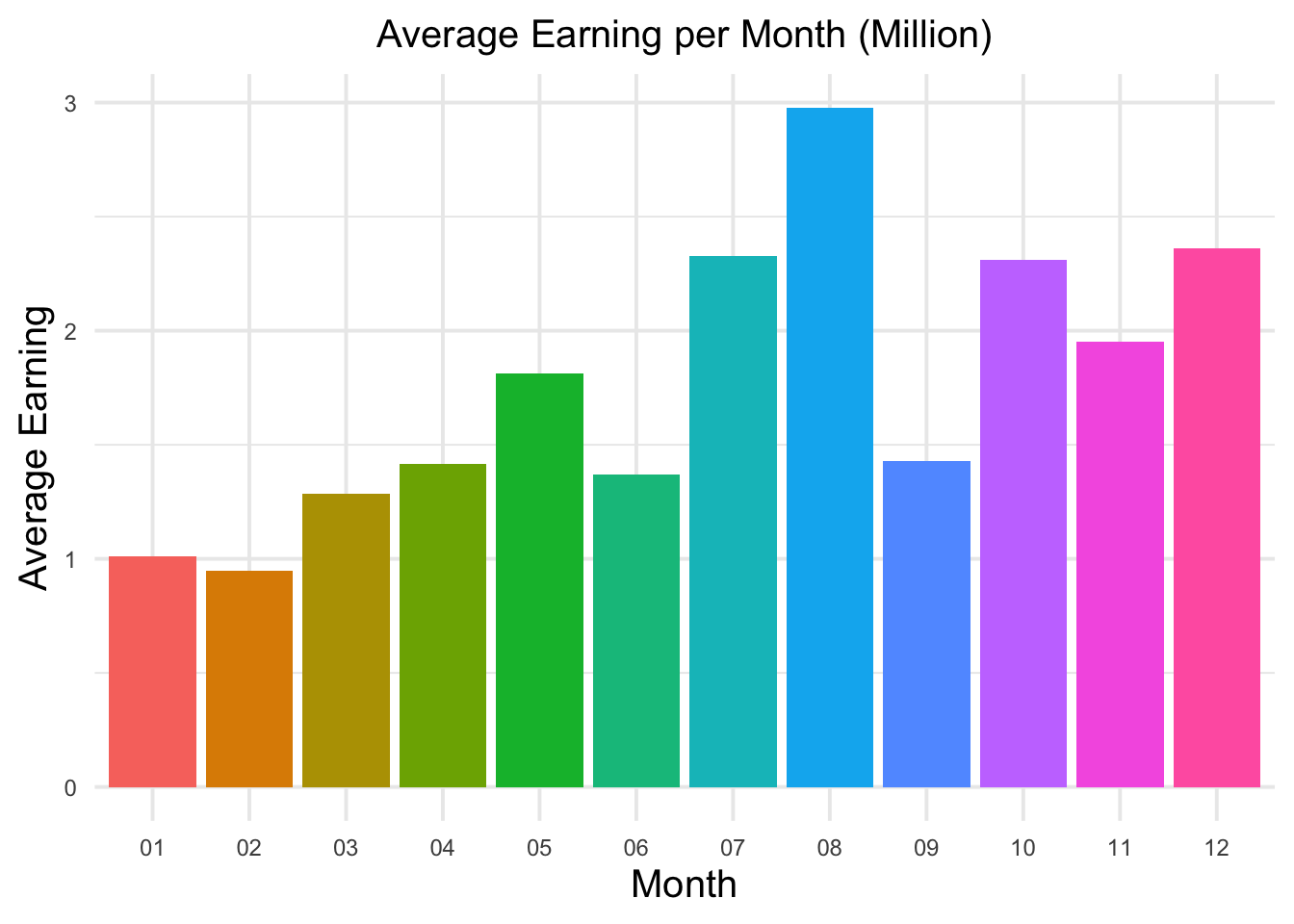
Q2(1) asks for the average earning per month. To answer this question, I first extracted the month from the date column in the dataset. Then, I grouped the data by month and calculated the average earnings for each month.
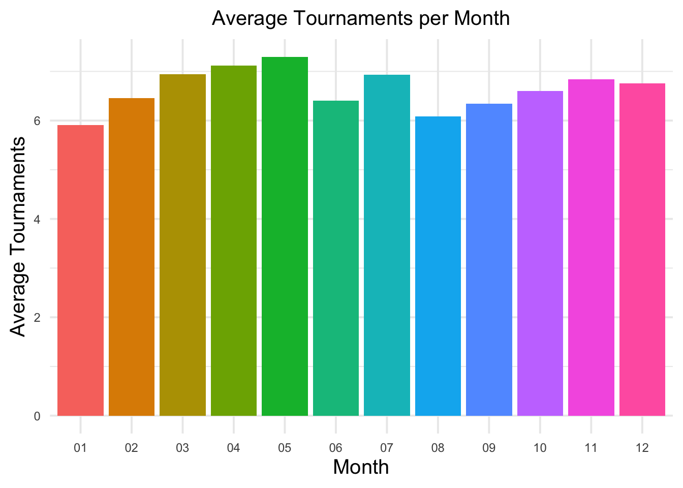
Q2(2) asks for the average tournaments per month. To answer this question, I first extracted the month from the date column in the dataset. Then, I grouped the data by month and calculated the average tournaments for each month.
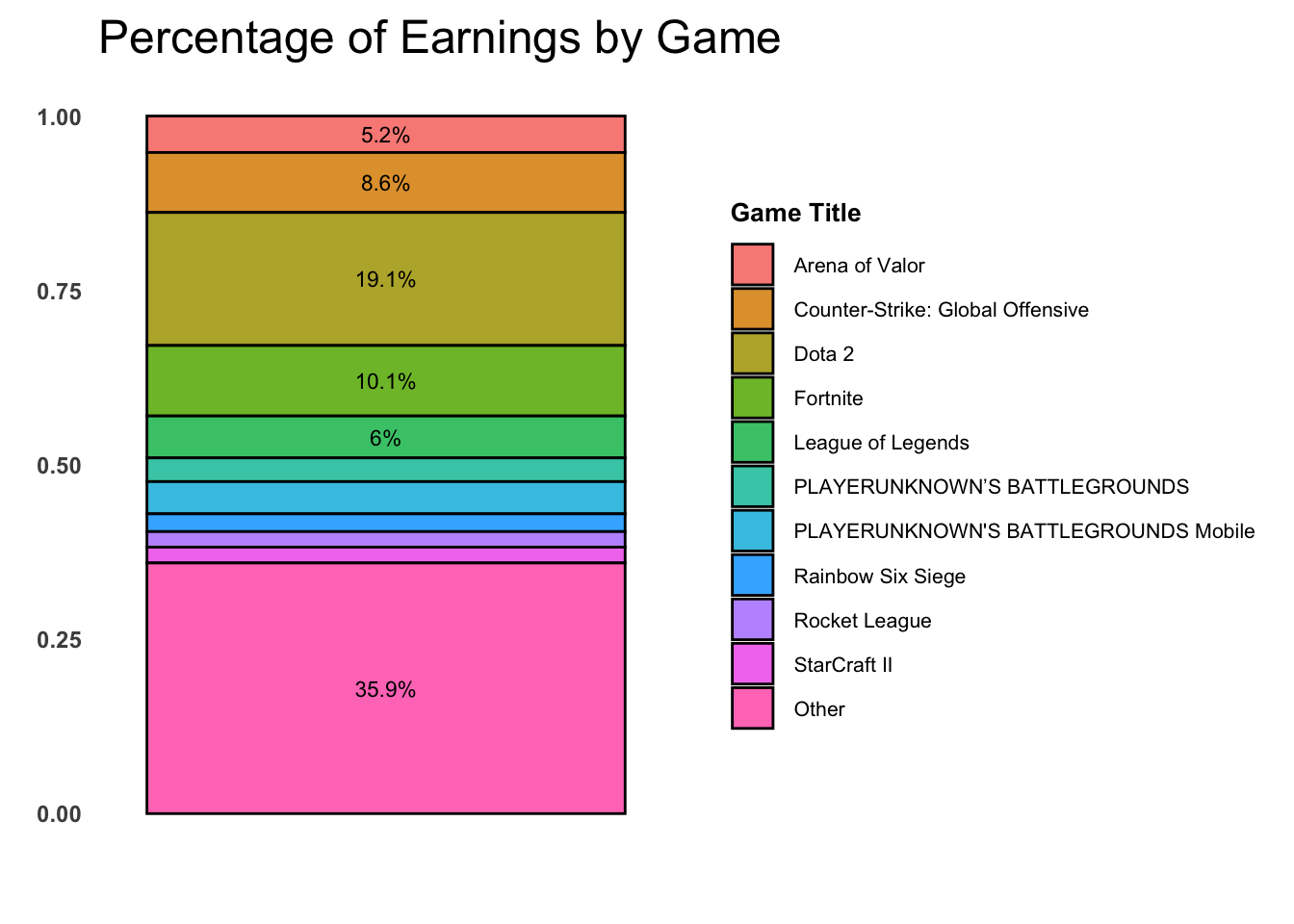
Q3 asks for the ten most profitable e-sport games. I first arranged the dataset in descending order based on the total earnings, which allowing me to sort the games by their profitability. Then I selected the top ten entries from the sorted dataset to identify the most profitable e-sport games.
The revenue of the ten most profitable e-sport games changed per years
Q4 asks how the revenue of the ten most profitable e-sport games changed over time. I first extracted the year from the date column in the dataset. Then, I filtered the data to include only the top 10 games identified in Q3. After that, I calculated the total earnings for each game in each year.
df_historical_cleaned |>mutate(year =year(date)) |>filter(game2 %in%c("Dota 2", "Fortnite", "Counter-Strike: Global Offensive", "League of Legends", "Arena of Valor", "PLAYERUNKNOWN'S BATTLEGROUNDS Mobile", "PLAYERUNKNOWN’S BATTLEGROUNDS", "Rainbow Six Siege", "StarCraft II", "Rocket League")) |>group_by(year, game2) |>summarise(earn_sum =sum(earn))
`summarise()` has grouped output by 'year'. You can override using the
`.groups` argument.
# A tibble: 97 × 3
# Groups:   year [14]
    year game2                            earn_sum
   <dbl> <chr>                               <dbl>
 1  2010 League of Legends                  27943.
 2  2010 StarCraft II                      820839.
 3  2011 Dota 2                           1672768.
 4  2011 League of Legends                 527995.
 5  2011 StarCraft II                     3222428.
 6  2012 Counter-Strike: Global Offensive  222539.
 7  2012 Dota 2                           2087095.
 8  2012 League of Legends                4287337.
 9  2012 StarCraft II                     4237569.
10  2013 Counter-Strike: Global Offensive 1219039.
# ℹ 87 more rows
The average monthly revenue of the ten most profitable e-sport games
Q5 asks for the average monthly revenue of the ten most profitable e-sport games. I first extracted the month from the date column in the dataset. Then, I filtered the data to include only the top 10 games identified in Q3. After that, I grouped the data by month and game and calculated the average earnings for each game in each month.
df_historical_cleaned |>mutate(month =substr(date, 6, 7)) |>filter(game2 %in%c("Dota 2", "Fortnite", "Counter-Strike: Global Offensive", "League of Legends", "Arena of Valor", "PLAYERUNKNOWN'S BATTLEGROUNDS Mobile", "PLAYERUNKNOWN’S BATTLEGROUNDS", "Rainbow Six Siege", "StarCraft II", "Rocket League")) |>group_by(month, game2) |>summarise(month_earning =mean(earn))
`summarise()` has grouped output by 'month'. You can override using the
`.groups` argument.
# A tibble: 120 × 3
# Groups:   month [12]
   month game2                                month_earning
   <chr> <chr>                                        <dbl>
 1 01    Arena of Valor                             548178.
 2 01    Counter-Strike: Global Offensive           833441.
 3 01    Dota 2                                    1012297.
 4 01    Fortnite                                   447184.
 5 01    League of Legends                          167203.
 6 01    PLAYERUNKNOWN'S BATTLEGROUNDS Mobile      2230359.
 7 01    PLAYERUNKNOWN’S BATTLEGROUNDS              202073.
 8 01    Rainbow Six Siege                           85265.
 9 01    Rocket League                              172484.
10 01    StarCraft II                               144511.
# ℹ 110 more rows
The earn per tournament trend for the ten most profitable e-sport games through 2017 to 2023
Q6 asks about the earnings per tournament trend for the ten most profitable e-sport games from 2017 to 2023. I first filtered the dataset to include only the specified top 10 games. Then, I applied another filter to restrict the data to the years between 2017 and 2023. After that, I calculated the earnings per tournament for each game by dividing the total earnings by the number of tournaments.
`summarise()` has grouped output by 'date'. You can override using the
`.groups` argument.
# A tibble: 764 × 3
# Groups:   date [84]
   date       game2                            t_earning
   <date>     <chr>                                <dbl>
 1 2017-01-01 Counter-Strike: Global Offensive    84323.
 2 2017-01-01 Dota 2                             176639.
 3 2017-01-01 League of Legends                   11979.
 4 2017-01-01 Rainbow Six Siege                     100
 5 2017-01-01 Rocket League                         223.
 6 2017-01-01 StarCraft II                         9723.
 7 2017-02-01 Counter-Strike: Global Offensive    13988.
 8 2017-02-01 Dota 2                              48536.
 9 2017-02-01 League of Legends                   20416.
10 2017-02-01 Rainbow Six Siege                  100000
# ℹ 754 more rows
Plot
library(plotly)
Attaching package: 'plotly'
The following object is masked from 'package:ggplot2':

    last_plot
The following object is masked from 'package:stats':

    filter
The following object is masked from 'package:graphics':

    layout
Earning per Year
# Create the plot and assign it to a variabledf_historical_cleaned |>mutate(year_total =year(date)) |>filter(year_total !=2024) |>group_by(year_total) |>summarise(yearsum =sum(earn) /1000000) |>ggplot(aes(x = year_total, y = yearsum, fill =as.factor(year_total))) +geom_col() +labs(title ="Earning per Year (million)",x ="Year",y ="Earning") +theme_minimal(base_size =15) +theme(legend.position ="none",plot.title =element_text(hjust =0.5))
# Specifies the factor variable to be modified, then keeps the top 10 levels based on the earn, and makes the levels that are not in the top 10 combined into a new level called "Other".df_general_cleaned |>mutate(game =fct_lump_n(f = game1, n =10, w = totalearn, other_level ="Other")) |>group_by(game) |>summarise(earnings =sum(totalearn), .groups ='drop') |>mutate(proportion = earnings /sum(earnings), Game =fct_reorder(.f = game, .x = proportion, .fun = max, .desc =TRUE),Game =fct_relevel(.f = game, "Other", after =Inf)) |>ggplot(aes(x ="", y = proportion, fill = game)) +# geom_col(width =1, color ="black", alpha =0.85) +theme_minimal(base_size =15) +theme(legend.position ="right", legend.title =element_text(face ="bold",size =10),axis.text =element_text(face ="bold",size =9),plot.background =element_blank(),legend.text =element_text(size =8),panel.grid =element_blank()) +labs(title ="Percentage of Earnings by Game", y =element_blank(), x =element_blank(),fill ="Game Title") +geom_text(aes(label =ifelse(proportion >0.05, paste0(round(proportion, 3) *100, "%"), "")),position =position_stack(vjust =0.5), size =3)
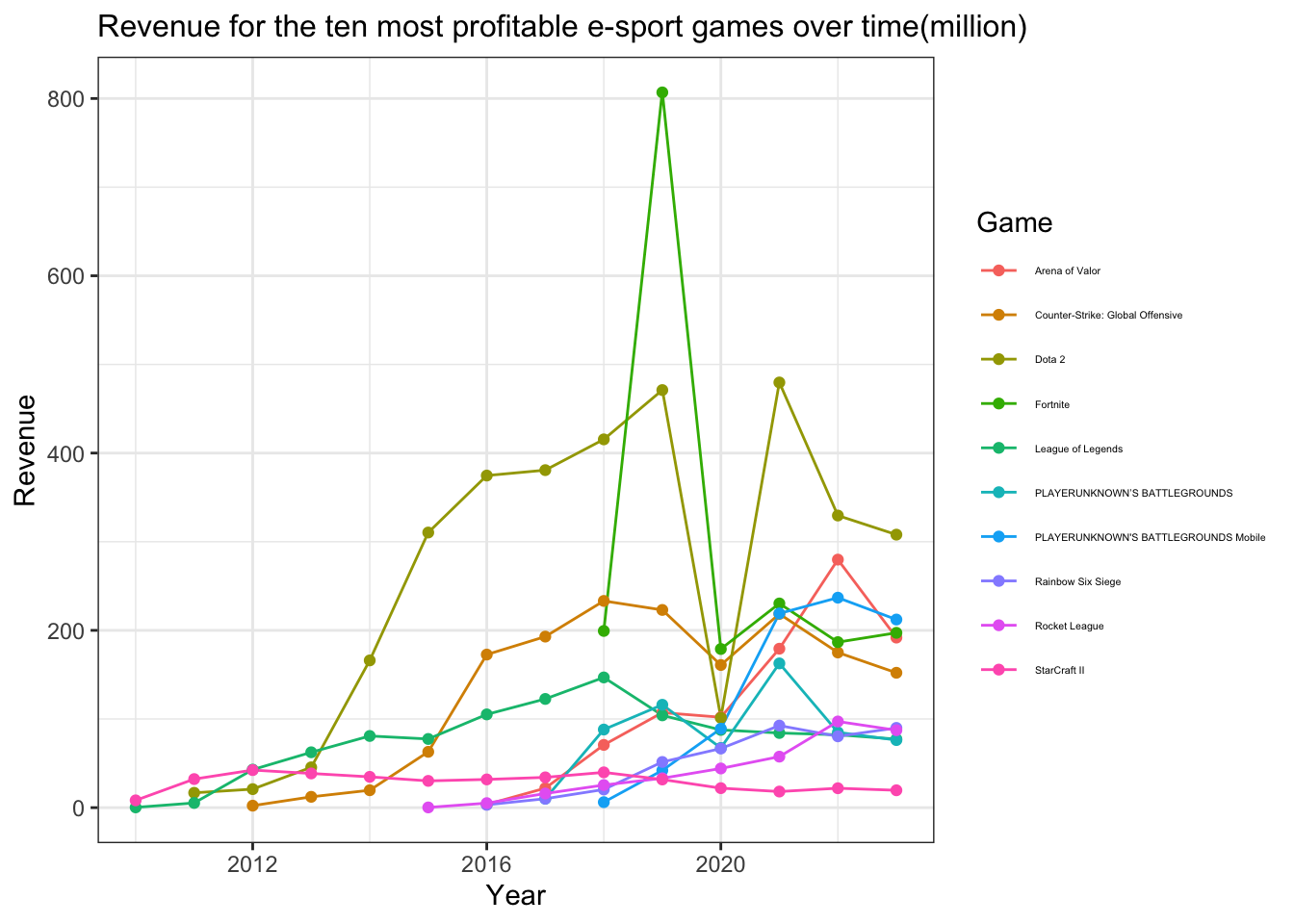
The revenue of the ten most profitable e-sport games changed per years
The ten most profitable e-sport games: Dota 2, Fortnite, Counter-Strike: Global Offensive, League of Legends, Arena of Valor, PLAYERUNKNOWN’S BATTLEGROUNDS Mobile, PLAYERUNKNOWN’S BATTLEGROUNDS, Rainbow Six Siege, StarCraft II, Rocket League
df_historical_cleaned |>mutate(year =year(date)) |>filter(year!=2024) |>filter(game2 %in%c("Dota 2", "Fortnite", "Counter-Strike: Global Offensive", "League of Legends", "Arena of Valor", "PLAYERUNKNOWN'S BATTLEGROUNDS Mobile", "PLAYERUNKNOWN’S BATTLEGROUNDS", "Rainbow Six Siege", "StarCraft II", "Rocket League")) |>group_by(year, game2) |>summarise(earn_sum =sum(earn)/100000) |>ggplot(aes(x = year, y = earn_sum, color = game2)) +geom_line() +geom_point() +labs(title ="Revenue for the ten most profitable e-sport games over time(million)",x ="Year",y ="Revenue",color ="Game") +theme_bw() +theme(legend.position ="right",legend.text =element_text(size =4),plot.title =element_text(size =12))
`summarise()` has grouped output by 'year'. You can override using the
`.groups` argument.
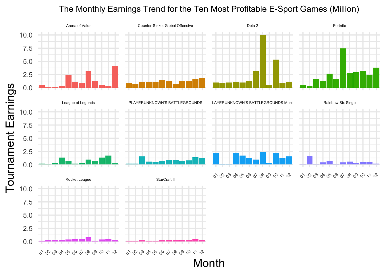
The average monthly revenue of the ten most profitable e-sport games
df_historical_cleaned |>mutate(month =substr(date, 6, 7)) |>filter(game2 %in%c("Dota 2", "Fortnite", "Counter-Strike: Global Offensive", "League of Legends", "Arena of Valor", "PLAYERUNKNOWN'S BATTLEGROUNDS Mobile", "PLAYERUNKNOWN’S BATTLEGROUNDS", "Rainbow Six Siege", "StarCraft II", "Rocket League")) |>group_by(month, game2) |>summarise(month_earning =mean(earn)/1000000) |>ggplot(aes(x = month, y = month_earning, fill = game2)) +geom_col() +facet_wrap(~game2) +labs(title ="The Monthly Earnings Trend for the Ten Most Profitable E-Sport Games (Million)",x ="Month",y ="Tournament Earnings",color ="Game") +theme_minimal(base_size =15) +theme(axis.text.x =element_text(size =6, angle =45, hjust =1),axis.text.y =element_text(size =9),plot.title =element_text(size =11, hjust =0.5),strip.text =element_text(size =5), legend.position ="none")
`summarise()` has grouped output by 'month'. You can override using the
`.groups` argument.
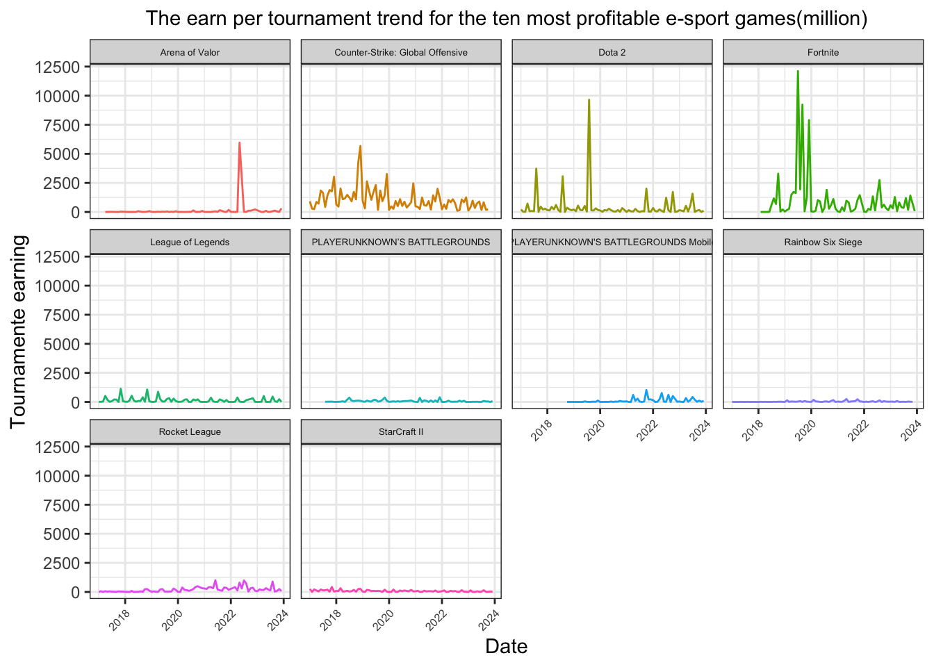
The earn per tournament trend for the ten most profitable e-sport games through 2017 to 2023
df_historical_cleaned |>filter(game2 %in%c("Dota 2", "Fortnite", "Counter-Strike: Global Offensive", "League of Legends", "Arena of Valor", "PLAYERUNKNOWN'S BATTLEGROUNDS Mobile", "PLAYERUNKNOWN’S BATTLEGROUNDS", "Rainbow Six Siege", "StarCraft II", "Rocket League")) |>filter(substr(date, 1, 4) %in%c("2017", "2018", "2019", "2020", "2021", "2022", "2023")) |>group_by(date, game2) |>summarise(t_earning = earn/100000*tournament) |>ggplot(aes(x = date, y = t_earning, color = game2)) +geom_line() +facet_wrap(~game2) +labs(title ="The earn per tournament trend for the ten most profitable e-sport games(million)",x ="Date",y ="Tournamente earning",color ="Game") +theme_bw() +theme(axis.text.x =element_text(size =6, angle =45, hjust =1),axis.text.y =element_text(size =9),plot.title =element_text(size =11, hjust =0.5),strip.text =element_text(size =5), legend.position ="none")
`summarise()` has grouped output by 'date'. You can override using the
`.groups` argument.